Download R Package From Schoam
![]()
By , Executive Editor, Data & Analytics, Computerworld |
About |
The focus here is on data: from R tips to desktop tools to taking a hard look at data claims.
Useful new R packages for data visualization and analysis
The following is from a hands-on session I led at the recent Computer Assisted Reporting conference.
There's a lot of activity going on with R packages now because of a new R development package called htmlwidgets, making it easy for people to write R wrappers for existing JavaScript libraries.
The first html-widget-inspired package I want us to demo is
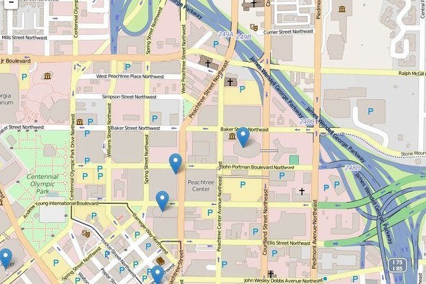
Leaflet for R.
If you're not familiar with Leaflet, it's a JavaScript mapping package. To install it, you need to use the devtools package and get it from GitHub (if you don't already have devtools installed on your system, download and install it with install.packages("devtools").
devtools::install_github("rstudio/leaflet") Load the library
library("leaflet") Step 1: Create a basic map object and add tiles
mymap <- leaflet() mymap <- addTiles(mymap) View the empty map by typing the object name:
mymap Step 2: Set where you want the map to be centered and its zoom level
mymap <- setView(mymap, -84.3847, 33.7613, zoom = 17) mymap Add a pop-up
addPopups(-84.3847, 33.7616, 'Data journalists at work, <b>NICAR 2015</b>') And now I'd like to introduce you to a somewhat new chaining function in R: %>%
This takes the results of one function and sends it to the next one, so you don't have to keep repeating the variable name you're storing things, similar to the one-character Unix pipe command. We could compact the code above to:
mymap <- leaflet() %>% addTiles() %>% setView(-84.3847, 33.7613, zoom = 17) %>% addPopups(-84.3847, 33.7616, 'Data journalists at work, <b>NICAR 2015</b>') View the finished product:
mymap Or if you didn't want to store the results in a variable for now but just work interactively:
leaflet() %>% addTiles() %>% setView(-84.3847, 33.7613, zoom = 16) %>% addPopups(-84.3847, 33.7616, 'Data journalists at work, <b>NICAR 2015</b>') Now let's do something a little more interesting - map nearby Starbucks locations. Load the starbucks.csv data set – See data source at: https://opendata.socrata.com/Business/All-Starbucks-Locations-in-the-US-Map/ddym-zvjk
Data files for these exercises are available on my NICAR15data repository on GitHub. You can also download the Starbucks data file directly from Socrata's OpenData site in R with the code
download.file("https://opendata.socrata.com/api/views/ddym-zvjk/rows.csv?accessType=DOWNLOAD", destfile="starbucks.csv", method="curl") starbucks <- read.csv("https://opendata.socrata.com/api/views/ddym-zvjk/rows.csv?accessType=DOWNLOAD", stringsAsFactors = FALSE) str(starbucks) atlanta <- subset(starbucks, City == "Atlanta" & State == "GA") leaflet() %>% addTiles() %>% setView(-84.3847, 33.7613, zoom = 16) %>% addMarkers(data = atlanta, lat = ~ Latitude, lng = ~ Longitude,popup = atlanta$Name) %>% addPopups(-84.3847, 33.7616, 'Data journalists at work, <b>NICAR 2015</b>') A script created by a TCU prof lets you create choropleth maps of World Bank data with a single line of code! More info here:
http://rpubs.com/walkerke/wdi_leaflet
We don't have time to do more advanced work with Leaflet, but you can do considerably more sophisticated GIS work with Leaflet and R. More on that at the end of this post.
More info on the Leaflet project page http://rstudio.github.io/leaflet/
A little more fun with Starbucks data: How many people are there per Starbucks in each state? Let's load in a file of state populations
statepops <- read.csv("acs2013_1yr_statepop.csv", stringsAsFactors = FALSE) # A little glimpse at the dplyr library; lots more on that soon library(dplyr) There's a very easy way to count Starbucks by state with dplyr's count function format: count(mydataframe, mycolumnname)
starbucks_by_state <- count(starbucks, State) We'll need to add state population here. You can do that with base R's merge or dplyr's left_join. left_join is faster but I find merge more intuitive
starbucks_by_state <- merge(starbucks_by_state, statepops, all.x = TRUE, by.x="State", by.y="State") # No need to do by.x and by.y if columns have the same name # better names names(starbucks_by_state) <- c("State", "NumberStarbucks", "StatePopulation") Add new column to starbucks_by_state with dplyr mutate function, which just means alter the data frame by adding one or more columns. Then we'll store in a new dataframe, starbucks_data, so as not to much with the original.
starbucks_data <- starbucks_by_state %>% mutate( PeoplePerStarbucks = round(StatePopulation / NumberStarbucks) ) %>% select(State, NumberStarbucks, PeoplePerStarbucks) %>% arrange(desc(PeoplePerStarbucks)) Again the %>% character, so we don't have to keep writing things like
starbucks_data <- mutate(starbucks_by_state, PeoplePerStarbucks = round(StatePopulation / NumberStarbucks)) starbucks_data <- select(starbucks_data, State, NumberStarbucks, PeoplePerStarbucks) starbucks_data <- arrange(starbucks_data, desc(PeoplePerStarbucks)) Can we pretend for a moment that doing a histogram of this data is meaningful :-)? Because I want to show you a cool new histogram tool in Hadley Wickham's ggvis package, still under development:
library(ggvis) starbucks_data %>% ggvis(x = ~PeoplePerStarbucks, fill := "gray") %>% layer_histograms() Not a big deal? How about one with interactive sliders?
starbucks_data %>% ggvis(x = ~PeoplePerStarbucks, fill := "gray") %>% layer_histograms(width = input_slider(1000, 20000, step = 1000, label = "width")) # Can even add a rollover tooltip starbucks_data %>% ggvis(x = ~PeoplePerStarbucks, fill := "gray") %>% layer_histograms(width = input_slider(1000, 20000, step = 1000, label = "width")) %>% add_tooltip(function(df) (df$stack_upr_ - df$stack_lwr_)) Time Series Graphing
Load needed libraries: dygraphs and xts if not on your system yet, first install with
install.packages("dygraphs") install.packages("xts") To begin, let's run some demo code with a sample data set already included with R, monthly male and female deaths from lung diseases in the UK from 1974 to 1979 datasets are mdeaths and fdeaths
First we'll create a single object from the two of them with the cbind() – combine by column – function.
library("dygraphs") library("xts") lungDeaths <- cbind(mdeaths, fdeaths) # And now here's how easy it is to create an interactive multi-series graph: dygraph(lungDeaths) The most "complicated" thing about dygraphs is that it is specifically for time series graphing and requires a time series object. You can create one with the base R ts() function
ts(datafactor, frequency of measurements per year, starting date as c(year, month))
Read in a data file on Atlanta unemployment rates
atl_un <- read.csv("FRED-ATLA-unemployment.csv", stringsAsFactors = FALSE) # now we need to convert this into a time series atl_ts <- ts(data=atl_un$Unemployment, frequency = 12, start = c(1990, 1)) dygraph((atl_ts), main="Monthly Atlanta Unemployment Rate") More info on dygraphs: http://rstudio.github.io/dygraphs
Note: There is an existing package called quantmod that will pull a lot of financial and economic data for you and put it into xts format. It pulls data from the Federal Reserve of St. Louis. I searched on their website and found out that the URL for Atlanta unemployment was
https://research.stlouisfed.org/fred2/series/ATLA013URN
which means the code is ATLA013URN
library("quantmod") This command
getSymbols("ATLA013URN", src="FRED") automatically pulls the data into R in the right time-series format, storing it in a variable the same name as the symbol, in this case ATLA013URN. Then we can use dygraph:
dygraph(ATLA013URN, main="Atlanta Unemployment") To change name of data column in the ATLA013URN time series:
names(ATLA013URN) <- "rate" Now re-graph:
dygraph(ATLA013URN, main="Atlanta Unemployment") Aside: Quantmod has its own data visualization if you're just exploring:
chartSeries(ATLA013URN, subset="last 10 years") Another very new package lets you do more exploring of FRED data from the Federal Reserve of St. Louis; you need a free API key from the Federal Reserve site. More info here
https://github.com/jcizel/FredR
There's another new package rbokeh, implementing an R version of the Python bokeh interactive Web plotting library. I'm going to skip this one since so much else to go over, but wanted you to know about it. It's still under development already well documented at
http://hafen.github.io/rbokeh/rd.html
One other htmlwidgets-inspired package:
library(DT) datatable(atl_un) Posted by: khecoebhoeng.blogspot.com
Source: https://www.computerworld.com/article/2894448/useful-new-r-packages-for-data-visualization-and-analysis.html